NLP基础 - CheaSim Blog

NLP基础

nlp 深度学习基础

将每一个模型以

  1. 简单介绍
  2. 解决的问题
  3. 代码
  4. 优缺点
  5. 使用tips

来归类。比较现代的会分析分析。

tf-idf

全称(term frequency-inverse document frequency),TF指的是词频,IDF指的是逆文本频率指数。他们的计算公式如下:

$TF_w=\cfrac{N_w}{N}$,一个词在该句子中出现的频率。

$IDF_w=\log{\cfrac{Y}{Y_w+1}}$,$Y_w$是所有文档中包含该词的文档个数。+1是方式分母为0.

TF-IDF的思想在于,一个词如果在一段小文本中出现得越多,那么他对这段文本的权重就越大,但是如果在所有的文本中,他出现的次数都很多,就像计算信息熵一样,在所有情况下出现的概率很大时,那么词的信息就很少。所有使用IDF来抵消一些常用词的影响。综上,计算公式为

$TFIDF_w=TF_w \times IDF_w$

注意,对于不同的样本的同一个词,$TF$可能是不同的,但是$IDF$是相同的。

解决的问题

TF-IDF相当于在以前把关键字作为短文本表示的基础上加入了一个正则化,削弱了高频词的权重。在一些简单的文本匹配(对于给定的问题,与已知文本的词语将TFIDF加和得到相似度),文本分类上可以起到一定的效果。


代码

1
2
3
4
5
6
7
8
9
10
11
12
13
14
15
16
17
18
19
20
21
22
23
24
25
26
27
import numpy as np
class TFIDF(object):
def __init__(self, documents_list):
self.documents_list = documents_list
self.tf = []
self.idf = {}
df = {}
for document in documents_list:
temp = {}
for word in document:
temp[word] = temp.get(word, 0) + 1./len(document)
self.tf.append(temp)
# 出现过的词,都+1
for k in temp.keys():
df[k] = df.get(k, 0) + 1
for k, v in df.items():
self.idf[k] = np.log(len(documents_list) / (v + 1))
self.tfidf = []
for tf_sentence in self.tf:
temp = {}
for k, v in tf_sentence.items():
temp[k] = v * self.idf[k]
self.tfidf.append(temp)
tfidf = TFIDF(['I have a pen'.split(), 'I have an apple'.split(), 'Bang, apple pen'.split()])
print(tfidf.tf)
print(tfidf.idf)
print(tfidf.tfidf)

优点

  • 一种无监督的生成句子词语向量的方法。
  • 可以很快地找到一句话的关键字
  • 耗费的计算资源较少。

缺点

  • 句子向量,或者词语向量没有上下文信息,词语与词语之间的位置关系也没有融入到表示当中。
  • 会将生僻词作为关键词,但其实生僻词意义不大。
  • 人名地名比较难以区分。

https://zhuanlan.zhihu.com/p/113017752

ps: python dict是真好用。

word2vec

word2vec说明白了也就是和TFIDF一样的将词语使用一个$f(x)$映射到数值的向量空间当中。由于词语不像是像素点有着天然的数值表示,word2vec针对词语转化为计算机可以理解的表示。

word2vec的思想是一个词的意思由它旁边的词构成。就像老话说的好,物以类聚,人以群分。但其实word2vec的损失函数和模型解决的问题是有一点割裂开的。word2vec想解决的问题是生成稠密的word embedding,而优化损失函数的目的是让两个词在window下的关系符合文本。损失函数是想,在一个窗口下,如果我中心词是”帅哥”,那么模型应该能推测前两个词是”我”和”是”。因为在样本中”我是帅哥”出现过很多次。之后由于损失函数的计算中,预测的条件概率是通过词向量的相似度来计算的,所以在优化模型中,也就达成了相似词汇产生相似词向量的目的。

word2vec又分为两种模型:

  1. skip-gram: 使用中心词周围的词来预测中心词。
  2. CBOW: 使用中心词来预测周围的词。

每一个词汇表示成为两个$d$维的向量,用来计算条件概率。$v_i \in \mathbb{R^d}$.之后每一个window下在中心词预测上下文的条件概率就是。

$$P(O=o|C=c)=\cfrac{\exp(u_o^Tv_c)}{\sum_{w \in Vocab} \exp(u_w^Tv_c)}$$

使用极大似然估计就是,$L(\theta)=\prod_{t=1}^T \prod_{-m \leq j \leq m ,j \neq 0} P(w_{t+j} | w_t; \theta)$

之后对极大似然估计常规操作,取log再正负相反,从而作为损失函数求最小。

![image-20210113160811012](/Users/cheasim/Library/Application Support/typora-user-images/image-20210113160811012.png)

$W_{V\times N}$就是由中心词汇组成的矩阵,$W’_{N \times V}$就是上下文词汇表示组成的矩阵。

skip gram

每一个词汇表示成为两个$d$维的向量,用来计算条件概率。$v_i \in \mathbb{R^d}$.这里我们直接想象成深度学习的模型,那么我们的输入是一个one hot embedding,输出是维度为词表的向量。之后我们要使得向量在上下文词上的值接近为1(在激活归一化之后)。由于词表一般很长,所以训练skip gram的时候有一个trick。

CBOW

使用平均加权的one hot embedding输入上下文词汇,去预测中心词汇。

Hierarchical Softmax

对于整个词表计算一次softmax的开销是很大的$O(|V|)$其中$|V|>>|d|$,所以我们需要构建一种不一样的softmax来处理这个问题。这个就是Hierarchical softmax 等级制的softmax,它首先会将词表进行分层,构建成一颗平衡二叉树,🌲上的节点就是我们要判断的word,我们知道平衡二叉树的深度是$O(\log n)$。经过$\log n$次的判断之后,就可以计算损失函数了。一次forward复杂度是$O(\log |V| * d2)$,其中2是在左右选择,相比于$O(|V|+d|V|)$减少了很多。计算P需要把从根节点到叶子节点上的每个节点挨个算一遍概率。

![image-20210113164654789](/Users/cheasim/Library/Application Support/typora-user-images/image-20210113164654789.png)

negative sampling

在一次训练的时候,skip gram 只会输入一个词,很稀疏,浪费了其他的embedding训练。在训练的时候,不使用矩阵直接乘,而是使用挑选比如(1+10)10个负样本更新矩阵。挑选的公式为出现评率比较大的。

$$P(w_i)=\cfrac{f(w_i)^{0.75}}{\sum_{j=0}^nf(w_j)^{0.75}}$$

解决的问题

解决one-hot embedding中过于稀疏,以及难以表达语义特征的问题。


代码

1
2
3
class Word2Vec(object):
def __init__(self, documents_list):


优点

  • 无监督训练生成词向量

  • 对于相似的词汇有着很好的解释性,Man - King = Woman - Queen

缺点

  • 无法一词多义。

  • 训练时没有加入位置信息,训练效率较低。

text-cnn

Convolutional Naural Networks for Sentence Classification

拷贝忍者卡卡sei,直接抄CV的CNN就完事了。我们可以将一句话利用word embedding看成是一副图像,比如长度为10的句子,词向量维度为300。那么这个句子的输入就是$10 \times 300$的矩阵。之后我们就可以像图像一样处理文本了。

image-20210113173917546

模型可以分为三层。

  1. 输入层是一个$k \times n$的矩阵
  2. 卷积层与CV有一些区别,因为我们需要把词向量看做是一个整体,所以不会在横(纵?)方向上进行卷积,卷积窗口只会上下移动。核大小为$filter_size \times embedding_size$.文中定义filiter_size为[3,4,5]。将局部的信息聚合。每一个不同的卷积核都会生成不同的feature map,比如输入是$10 \times 300$,之后经过128个大小为3的卷积操作,会生成128个维度为10的向量。
  3. pooling层,由于要处理变长文本,所以是对每一个feature map上取最大值作为输出,所以最终得到的是一个128维度的向量。
  4. FFN和Softmax 常规操作,分类模型获得每一类的概率。

解决的问题

将CNN引入到NLP当中,从而减少了模型的参数,并在CNN在捕捉局部信息时有奇效。


1
2
3
4
5
import torch
import torch.nn as nn
class TextCNN(nn.Module):
def __init__(self,):
pass

优点

  • 跨时代地提出了CNN在NLP领域的应用
  • 实验做得很详细,针对预训练,随机生成的词向量都进行了比对。(是不是这个给bert一点思考,不需要一个word embedding,随机初始化就好了)

缺点

  • CNN卷积对于句子来说还是太小了。没有全局信息。一个CNN只能估计5-gram的信息

https://zhuanlan.zhihu.com/p/102426363

rnn lstm

RNN想对于CNN模型来说多了很多变种。首先来说一下RNN的思想吧。RNN灵感来源于人类进行阅读过程中,会从左到右一个字一个字地读入文字,之后再得到自己的理解。那么是否有模型能够捕捉这种从左到右的时序信息呢?那就是RNN(Recurrent Neural Network)。RNN由于结构精巧有很多变种。

rnn

LSTM

LSTM使用门机制来进行有效地方式了梯度爆炸或者梯度消失。他三个门的公式分别是输入门,遗忘门,输出门。

$f_i=$

http://codewithzhangyi.com/2018/10/31/NLP%E7%AC%94%E8%AE%B0-RNN/

transformer

BERT

代码来自transformers==3.3.1

input

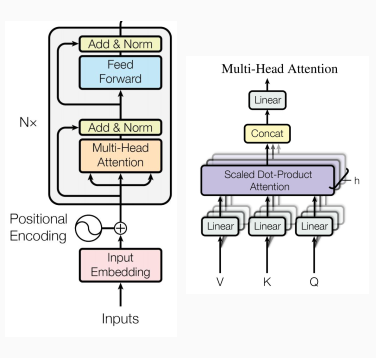
BERT模型的输入由三部分得到,token embdding, segment embedding, position embedding。

token embedding

对于所有文字来说,计算机都是无法理解的,需要转化为浮点向量或者整型向量。BERT采用的是WordPiece tokenization,是一种数据驱动的分词算法,他以char作为最小的粒度,不断地寻找出现最多以char为单位组成的token,之后将word进行分词,分为一个一个的token。比如ing这个会经常出现在英文当中,所以WordPiece 会吧”I am playing the computer games”分为”I am play ##ing the computer games”。为了解决OOV问题。词表中有30522个词。

在WordPiece 分词的基础上,之后会加入4个特殊词汇[CLS],[SEP],[PAD],[UNK]。[CLS]加入到句首,不参与预训练,针对下游任务进行fine-tune。[SEP]作为句尾以及分段标志。[PAD]是填充,使得句子长度一样,方便批处理,[UNK]是表明不在词表当中。将他们转换成one-hot embedding之后,接一个embedding层,将词转化为最初的词向量。

segment embedding

segment embedding 仅仅作为区分两个句子来使用。在预训练中,还要使用预测句子是否相邻作为预训练任务之一。在输入时,也会经过一个线性层来形成segment embedding.

position embedding

position embedding 纯使用nn.embedding 获得。训练了一个位置词表。$W\in \mathbb{R^{512 \times 768}}$。输入就是[0,1,2,…,len_seq-1]

1
2
3
4
5
6
7
8
9
10
11
12
13
14
15
16
17
18
19
20
21
22
23
24
25
26
27
28
29
30
31
32
33
34
35
36
37
38
39
class BertEmbeddings(nn.Module):
"""Construct the embeddings from word, position and token_type embeddings."""
def __init__(self, config):
super().__init__()
self.word_embeddings = nn.Embedding(config.vocab_size, config.hidden_size, padding_idx=config.pad_token_id)
self.position_embeddings = nn.Embedding(config.max_position_embeddings, config.hidden_size)
self.token_type_embeddings = nn.Embedding(config.type_vocab_size, config.hidden_size)

# self.LayerNorm is not snake-cased to stick with TensorFlow model variable name and be able to load
# any TensorFlow checkpoint file
self.LayerNorm = nn.LayerNorm(config.hidden_size, eps=config.layer_norm_eps)
self.dropout = nn.Dropout(config.hidden_dropout_prob)

# position_ids (1, len position emb) is contiguous in memory and exported when serialized
self.register_buffer("position_ids", torch.arange(config.max_position_embeddings).expand((1, -1)))
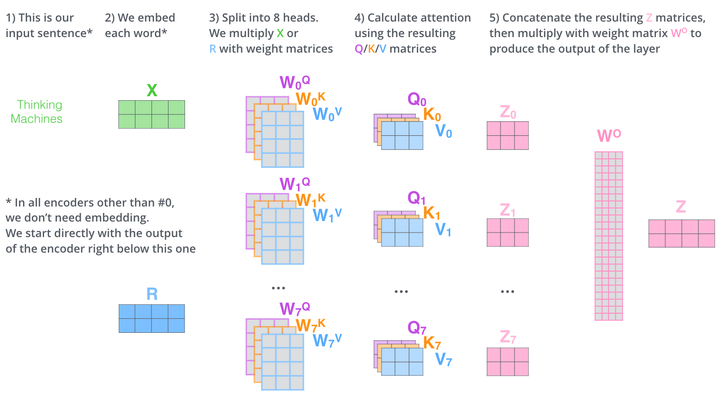
def forward(self, input_ids=None, token_type_ids=None, position_ids=None, inputs_embeds=None):
if input_ids is not None:
input_shape = input_ids.size()
else:
input_shape = inputs_embeds.size()[:-1]

seq_length = input_shape[1]

if position_ids is None:
position_ids = self.position_ids[:, :seq_length]

if token_type_ids is None:
token_type_ids = torch.zeros(input_shape, dtype=torch.long, device=self.position_ids.device)

if inputs_embeds is None:
inputs_embeds = self.word_embeddings(input_ids)
position_embeddings = self.position_embeddings(position_ids)
token_type_embeddings = self.token_type_embeddings(token_type_ids)

embeddings = inputs_embeds + position_embeddings + token_type_embeddings
embeddings = self.LayerNorm(embeddings)
embeddings = self.dropout(embeddings)
return embeddings

transformer encoder 层

transformer encoder层主要如下图所示

image

使用一个上面所说的输入,经过Multi-Head Attention,在通过残差连接以及Layer Normalization,之后通过FFN以及又一个残差连接作为输出。

Multi-Head Attention

BERT使用的是自注意力机制,即用于$Q,K,V$全部源自同一个向量。注意力机制使用了上下文的信息来对每一个token进行表示。计算机通过利用上下文的信息,对每一个token进行理解。比如“冬天到了,天气变冷了。”BERT会根据大量该类的文本,将冬天和冷的语义进行融合。Attention值的计算公式如下

$$Attention(Q,K,V)=softmax(\cfrac{QK^T}{\sqrt{d_k}})V \in \mathbb{R^{len\times d}}$$

其中,$Q,K,V\in \mathbb{R^{d\times k}},Q=xW_q,K=xW_k,V=xW_v$,$d$是隐层维度这里可以注意到,因为softmax是非线性的,所以这里的矩阵变换是没法单纯使用线性变换用$Wx$代替的。


多头在哪里多头。直接将原来的$x$进行转化后切分,详情看下图就懂了。每一个attention生成的维度都不高,拼起来就跟原来一样了。这张图有点问题,其实BERT没有$W^O$,因为$Z_0,…,Z_7$拼起来正好是$Z$。

img1

BERT 实现中,多头的目的是降低参数的个数,增加表达能力。 类似于CNN多个卷积核?

1
2
3
4
5
6
7
8
9
10
11
12
13
14
15
16
17
18
19
20
21
22
23
24
25
26
27
28
29
30
31
32
33
34
35
36
37
38
39
40
41
42
43
44
45
46
47
48
49
50
51
52
53
54
55
56
57
58
59
60
61
62
63
64
65
66
67
68
69
70
71
72
73
74
75
76
class BertSelfAttention(nn.Module):
def __init__(self, config):
super().__init__()
if config.hidden_size % config.num_attention_heads != 0 and not hasattr(config, "embedding_size"):
raise ValueError(
"The hidden size (%d) is not a multiple of the number of attention "
"heads (%d)" % (config.hidden_size, config.num_attention_heads)
)

self.num_attention_heads = config.num_attention_heads
self.attention_head_size = int(config.hidden_size / config.num_attention_heads)
self.all_head_size = self.num_attention_heads * self.attention_head_size

self.query = nn.Linear(config.hidden_size, self.all_head_size)
self.key = nn.Linear(config.hidden_size, self.all_head_size)
self.value = nn.Linear(config.hidden_size, self.all_head_size)

self.dropout = nn.Dropout(config.attention_probs_dropout_prob)

def transpose_for_scores(self, x):
new_x_shape = x.size()[:-1] + (self.num_attention_heads, self.attention_head_size)
x = x.view(*new_x_shape)
return x.permute(0, 2, 1, 3)

def forward(
self,
hidden_states,
attention_mask=None,
head_mask=None,
encoder_hidden_states=None,
encoder_attention_mask=None,
output_attentions=False,
):
mixed_query_layer = self.query(hidden_states)

# If this is instantiated as a cross-attention module, the keys
# and values come from an encoder; the attention mask needs to be
# such that the encoder's padding tokens are not attended to.
if encoder_hidden_states is not None:
mixed_key_layer = self.key(encoder_hidden_states)
mixed_value_layer = self.value(encoder_hidden_states)
attention_mask = encoder_attention_mask
else:
mixed_key_layer = self.key(hidden_states)
mixed_value_layer = self.value(hidden_states)

query_layer = self.transpose_for_scores(mixed_query_layer)
key_layer = self.transpose_for_scores(mixed_key_layer)
value_layer = self.transpose_for_scores(mixed_value_layer)

# Take the dot product between "query" and "key" to get the raw attention scores.
attention_scores = torch.matmul(query_layer, key_layer.transpose(-1, -2))
attention_scores = attention_scores / math.sqrt(self.attention_head_size)
if attention_mask is not None:
# Apply the attention mask is (precomputed for all layers in BertModel forward() function) [1,1,1,0,0] -> [0,0,0,-10000,-10000]
attention_scores = attention_scores + attention_mask

# Normalize the attention scores to probabilities.
attention_probs = nn.Softmax(dim=-1)(attention_scores)

# This is actually dropping out entire tokens to attend to, which might
# seem a bit unusual, but is taken from the original Transformer paper.
attention_probs = self.dropout(attention_probs)

# Mask heads if we want to
if head_mask is not None:
attention_probs = attention_probs * head_mask

context_layer = torch.matmul(attention_probs, value_layer)

context_layer = context_layer.permute(0, 2, 1, 3).contiguous()
new_context_layer_shape = context_layer.size()[:-2] + (self.all_head_size,)
context_layer = context_layer.view(*new_context_layer_shape)

outputs = (context_layer, attention_probs) if output_attentions else (context_layer,)
return outputs

ps: 代码里实现attention_mask使用了加法,因为softmax中针对e^0也会输出1,所以我们要对于忽视的token进行$e^{-inf}$,才能使他在softmax之后的权重为0。

add and norm

常见的残差网络方式梯度消失,增加模型的训练,打破了网络的对称性,提升了网络的表征能力。

1
2
3
4
5
6
7
8
9
10
11
12
class BertSelfOutput(nn.Module):
def __init__(self, config):
super().__init__()
self.dense = nn.Linear(config.hidden_size, config.hidden_size)
self.LayerNorm = nn.LayerNorm(config.hidden_size, eps=config.layer_norm_eps)
self.dropout = nn.Dropout(config.hidden_dropout_prob)

def forward(self, hidden_states, input_tensor):
hidden_states = self.dense(hidden_states)
hidden_states = self.dropout(hidden_states)
hidden_states = self.LayerNorm(hidden_states + input_tensor)
return hidden_states

FFN and Add Norm

先经过中间层3072,hidden_size扩大4倍。之后再经过一个缩小了。注意这里最后才有一个dropout。激活函数用的gelu,比relu稍微缓和了一些。

1
2
3
4
5
6
7
8
9
10
11
12
13
14
15
16
17
18
19
20
21
22
23
24
25
26
class BertIntermediate(nn.Module):
def __init__(self, config):
super().__init__()
self.dense = nn.Linear(config.hidden_size, config.intermediate_size)
if isinstance(config.hidden_act, str):
self.intermediate_act_fn = ACT2FN[config.hidden_act]
else:
self.intermediate_act_fn = config.hidden_act

def forward(self, hidden_states):
hidden_states = self.dense(hidden_states)
hidden_states = self.intermediate_act_fn(hidden_states)
return hidden_states

class BertOutput(nn.Module):
def __init__(self, config):
super().__init__()
self.dense = nn.Linear(config.intermediate_size, config.hidden_size)
self.LayerNorm = nn.LayerNorm(config.hidden_size, eps=config.layer_norm_eps)
self.dropout = nn.Dropout(config.hidden_dropout_prob)

def forward(self, hidden_states, input_tensor):
hidden_states = self.dense(hidden_states)
hidden_states = self.dropout(hidden_states)
hidden_states = self.LayerNorm(hidden_states + input_tensor)
return hidden_states

最后处理

综上,把这个bert_layer叠个12层就行了。但是在最后输出的时候[CLS]有一个特殊的处理。输出的时候会经过一个线性层+一个tanh激活。

NER token classification

在每一个token对应的输出加入一个线性分类层,对应所有的实体类型标签比如B-PER,I-PER。

https://zhuanlan.zhihu.com/p/109250703

https://zhuanlan.zhihu.com/p/47282410

作者

CheaSim

发布于

2021-01-12

更新于

2021-03-08

许可协议

You forgot to set the business or currency_code for Paypal. Please set it in _config.yml.

评论